For a number of years, I taught a graduate-level course in project management. As one of the components of that course, student teams undertook a competitive exercise in which they would bid, plan, and then track the building of a 500-piece model (see Figure 1). The model is one that an apt nine-year-old could build in one and one-half hours following a well-defined sequence of steps specified in the manual. The student teams were comprised of a project manager and four or five builders. The challenge was to complete the project in the shortest amount of time, while maintaining the level of profit stated in their bids. Data collected from the exercise outcomes yields several interesting observations regarding project estimate error.
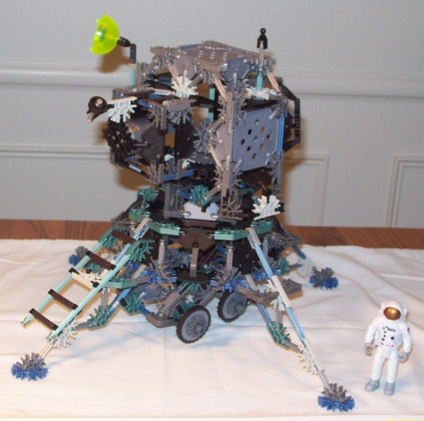
Figure 1. Apollo 15 Lunar Lander (K’nex model 13147).
The exercise
The exercise was based on the Project Management Simulation course developed by Eric Verzuh at The Versatile Company (2018). The timing and deliverables of the commercial, continuing-education course were modified extensively to fit an academic setting, including the use of software tools, homework and grading. The exercise involved three project phases: bid, plan and execution.
First, teams bid the project. Bids were evaluated in terms of shortest completion time (minutes) and least cost (dollars). The bids included labor and material costs. The bidding process was complicated by the fact that each team needed to subcontract with other teams to complete certain portions of the model. Bids could include contingency and management reserves. Teams would set a level of profit that would provide investment return while still keeping their bids competitive.
Second, teams prepared a project plan. While the manual defined a sequence of 66 steps that one nine-year old could follow in constructing the model, teams needed to determine which parts of the model could be built in parallel. This would take advantage of having more than one builder, and hence, allow them to shorten the build time. Defining the network diagram was a vital first step.
Teams needed to estimate the amount of time each step would take and how much it would cost. The labor cost rate was set at $1/minute of work, to keep the arithmetic simple. The labor cost represented the total amount of team effort. To prepare estimates, some teams chose to time the execution of certain steps. Based on a count of parts assembled in each step, they would use a part per minute average to estimate the duration of other steps. Other teams went to the trouble of buying a used kit on eBay, building the kit a number of times, and then fitting a learning curve to their build times in order to predict their overall execution time. (Yes, that was beyond what was expected. But, the exercise was part of their course grade.)
The project was resource constrained. If one had more than 25 builders at the outset, the model could be built in about 15 minutes, considering the number of parallel paths through the network diagram. The one and one-half hours one nine-year-old would take represented the other extreme. Each team had one project manager assigned to a level-of-effort task for the entire duration of the project. The other four or five team members were assigned to specific tasks throughout the project. This constrained the number of concurrent tasks at any one time. Each team needed to prepare a resource-leveled schedule (see Figure 2 for an example schedule excerpt). Towards the end of the schedule, utilization would drop-off as there were fewer concurrent tasks than there were resources. Teams were allowed to incorporate planned staff layoffs in their schedules. A modest cost penalty was imposed for a layoff relative to the proportion of total project duration the layoff represented.
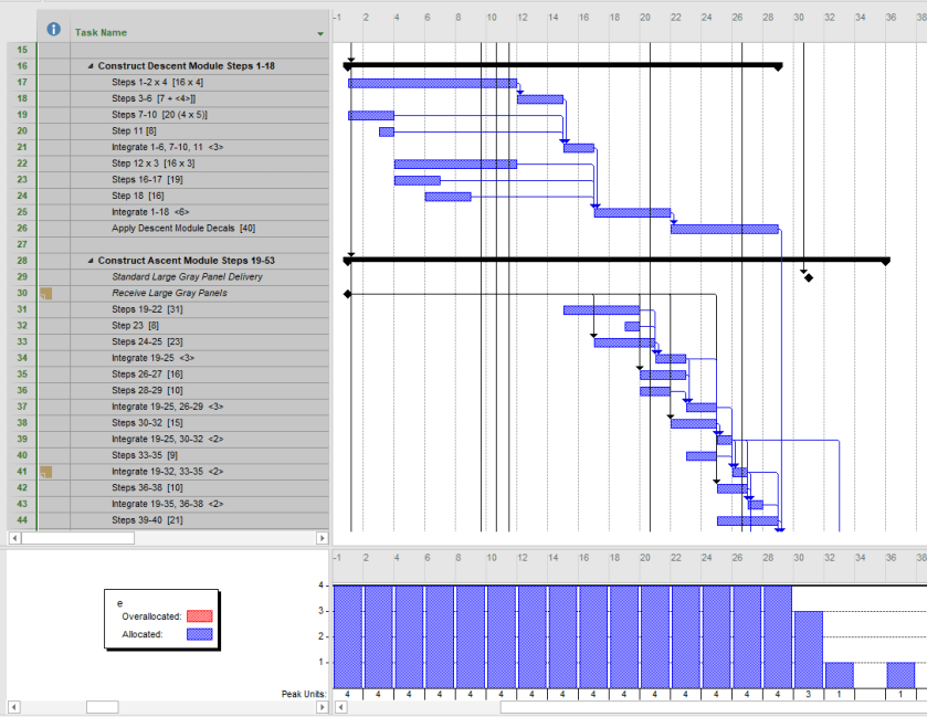
Figure 2. Excerpt of leveled schedule, showing utilization of four builders.
Once a team had a resource-leveled schedule, they had to baseline the project and present a cumulative cost curve against which they would track the project. Plans were evaluated on their components (task list, network diagram, basis of estimates, leveling and baseline). Once plans were submitted, teams were offered an optional performance bonus/penalty, a dollar amount per minute completed prior to or after the planned completion time.
Third, teams had to build the model according to plan, using earned value management techniques to periodically report project status. Each team had to prepare a tracking plan explaining what data they would collect, when and how. The build was partitioned into four equal time periods. Some teams completed the build within the second time period, while others required the full four periods. At the end of each period, teams reported project status and the results were posted (see Figure 3). Teams that maintained or improved their schedule and cost performance indices during project execution were viewed favorably. Teams had to explain variances in their performance.
Finally, at the end of the build, each team had to prepare a project profit and loss statement. Teams that met or exceeded their profit goals were viewed favorably.
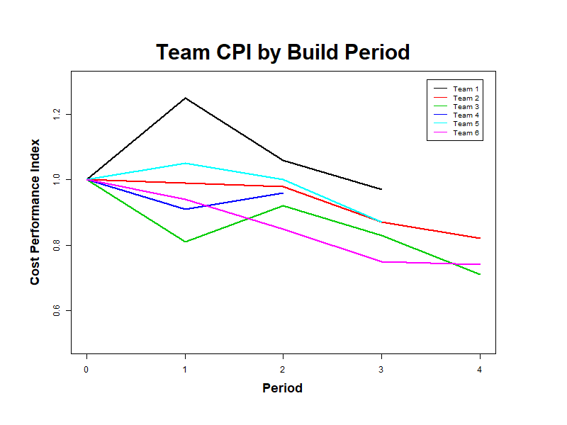
Figure 3. Example team CPI by build period chart
The data: bid, plan and actual
The course was offered ten times over a six-year period. Fifty-one teams competed in the exercise. For each team, the total project duration and labor cost were recorded from their bid, plan and execution documents. In this data set, for each team, there were three pairs of values, two estimates (bid and plan) and one actual. Each pair was comprised of a total project duration (minutes) and total labor cost (dollars).
Only labor costs will be compared across the three project phases. On average, labor costs represented 56% of the bid price. Labor costs were recorded separately in all three phases. Material and subcontractor costs were somewhat time invariant, whereas direct labor costs tended to vary with duration. Material and subcontractor costs were included in the bid and in the final profit and loss statement.
Confidence ellipses
Actual duration and labor cost were normally distributed. Taken together, they define a bivariate distribution. Figure 4 shows the prediction ellipse and confidence ellipse for the actual project duration and labor cost. The prediction ellipse shows the area within which we would expect a new, future value to occur 95% of the time. The confidence ellipse shows the area within which we are 95% confident the bivariate mean occurs. Across the 51 teams, the average time it took to build the model was 60.27 minutes and the average labor cost was $282.58.
Labor cost was positively correlated with project duration. The longer the project ran, labor costs were greater. This positive correlation held for bid and plan data, as well. This does not mean that there is a causal relationship between the two variables.
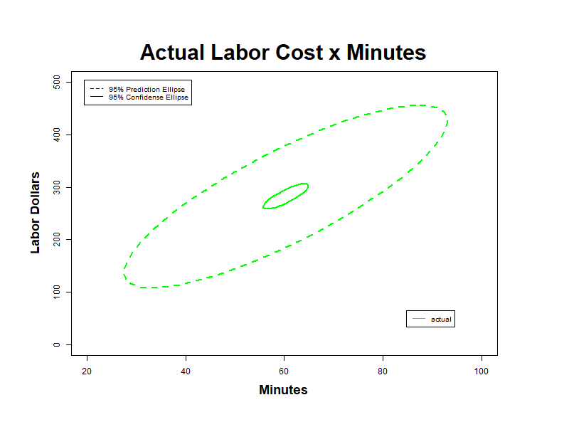
Figure 4. Actual labor cost by duration (Mean=<60.27 min, $282.58>).
When the prediction and confidence ellipses for the bid and plan phases are overlaid, several observations can be made (see Figure 5). First, the three distributions were significantly different. The confidence ellipses do not overlap. Second, total project duration was underestimated in the bid and more so in the plan. And third, total labor cost was underestimated in the plan. Interestingly, the plan estimates were less accurate than the bid estimates.

Figure 5. Bid, plan and actual labor cost by duration. 95% Prediction and 95% confidence ellipses. (Means: bid <52.5 min, $265.79>, plan <49.15 min, $223.14>, and actual <60.27 min, $282.58>).
The box plots in Figure 6 confirm these observations. Bid and plan duration were underestimated. The plan labor cost was underestimated.

Figure 6. Box plots showing labor cost and duration across bid, plan and execution phases
Estimate error
Estimate error is the difference between an actual value and an estimate. We would expect estimate errors to be normally distributed around zero. Estimate accuracy is the ratio of an actual value to an estimate (actual/estimate). We would expect estimate accuracy to be normally distributed around 1.0. In this case, the error accuracy distributions were normally distributed, but with means greater than 1.0. It is not uncommon for estimate accuracy distributions to be skewed towards larger errors. Once the one outlying bid labor cost estimate was removed, all of the estimate accuracy distributions were not significantly skewed.
Figure 7 shows box plots of labor cost and duration estimate accuracy, between the bid and plan phases. Plan estimate errors were significantly greater than bid errors. This is unexpected. Since the bid preceded the plan in this exercise, one might anticipate that the plan would be more accurate.
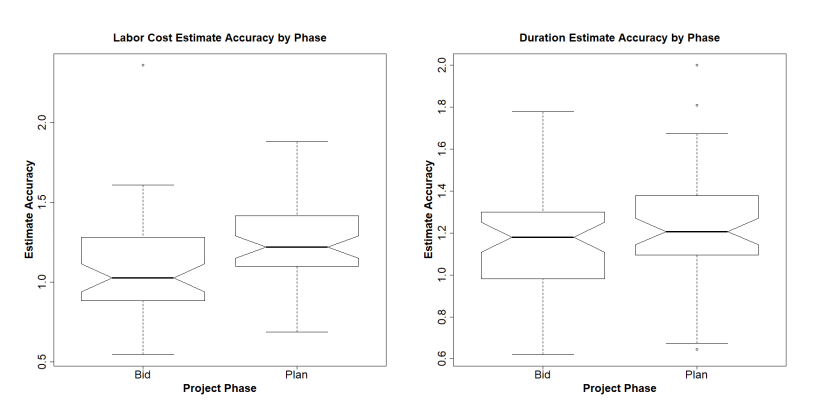
Figure 7. Labor cost and duration estimate accuracy by phase. Estimate accuracy means: bid duration=1.17, bid labor cost=1.08, plan duration=1.23, and plan labor cost=1.27
Figure 8 shows the confidence ellipses for the bid and plan estimate accuracies. The plan estimates were less accurate than the bids.

Figure 8. Bid and plan estimate accuracy confidence ellipses.
Discussion
Ideally, for this exercise, we would expect bids to be less accurate than plans, and that actual performance would be accurately forecast by the two estimates. That was not the case. However, the data collected does not permit exploration as to why the ideal was not met. Further investigation is needed. Still, several observations can be made and interesting questions posed.
In order to have this discussion, estimate and actual data had to be collected. Generally, projects are unique and we do not have data from which to make predictions about project outcomes. In this case, with data from 51 replications of the same project, statistical predictions about future, similar projects can be made. Further, estimate accuracy was measured. Estimate accuracy can only be improved if you can benchmark the current level of accuracy.
However, recording project data is difficult. Often, it is proprietary and cannot be shared. Since projects are disparate, it takes considerable work to scale and transform project data into a form in which cross-project comparisons can be made.
In lieu of data, project schedule and cost simulation techniques can be used to set confidence levels around estimates. However, these techniques depend upon assumptions regarding the uncertainty inherent in the estimates. Simulation models can be validated only if there is actual data to compare model results against.
There was variation in project execution. This variation represents the uncertainty we face when bidding and planning projects. One obvious cause of this variation is that some teams built faster than other teams. But, there may have been other confounding factors that are were not represented in the data. Further investigation is warranted. If your team was one of fifty teams undertaking the exact same project, how would your team’s execution compare with that of other teams, in terms of duration and cost?
There was variation in bid and plan estimates. Even though each team worked from the same specification, there were many different schedules and budgets. The schedules varied in terms of complexity. For example, plans varied in the number of tasks, in the number of task dependencies, and in resource utilization. And, there was variation in the methods used to estimate duration and cost. How did these factors contribute to the overall variation in the estimates and estimate accuracy?
If the distribution of actual project duration and cost were known, how would that influence selection of a bid? In this example, choosing the lowest bid in terms of cost, time, or both, would not have been a prudent choice. If there are confidence ellipses based on actual data from completed projects, we could assign a confidence level to a bid. Confidence levels could be used to screen bids.
The bid and plan estimates were not accurate. Both bids and plans were underestimates. In the real world, the reasons for inaccurate estimates might be fraud, greed, negligence, incompetence, or some combination of these reasons. In an academic setting, we would hope that these reasons do not apply. However, the desire to compete, coupled with inexperience, may have been biasing factors contributing to estimate inaccuracy.
Why were the plans more aggressive than the bids? As teams worked through their plans, did the increased familiarity with the tasks bias their estimates? This is an intriguing question. At this point, however, it is not possible to generalize the observation beyond the exercise and this data set.
References
Project Management Simulation. (2018). Versatile Company. Retrieved from http://www.versatilecompany.com/1project-management-simulation.aspx on 9 September 2018.
________________
© Nicklas, Inc. and robinnicklas.com, 2018. All rights reserved. Unauthorized use and/or duplication of this material without express and written permission from this site’s author and/or owner is strictly prohibited.
