Task criticality and finish time correlation in resource-constrained project schedule simulation

In a prior article, simulation techniques were used to explore the distribution of non-delay resource-feasible schedules and to identify resource critical paths (RCP’s).  Being able to identify RCP’s is useful since project schedule length in a resource-constrained schedule is driven by RCP’s and not the simple critical paths (CP’s) identified in its antecedent resource unconstrained schedule.  As was seen in the article, the expected project duration of a resource constrained schedule and its unconstrained antecedent can be very different.

A task’s criticality and finish time correlation are indicators of how much influence that task will have on the overall schedule duration.   Criticality measures the likelihood that a task will appear on a critical path.  Finish time correlation measures the relation between a task’s finish time and the project schedule’s finish time.  Just as the expected durations of the resource unconstrained and constrained project schedules can vary, criticality and finish time correlation will vary.  Hence, it is important that a project manager be able to assess these differences between the resource unconstrained and constrained schedules.   This article will illustrate these differences with an example.

Resource constraints and resource critical paths

Schedule duration in resource unconstrained schedules is driven by one or more critical paths, as computed using the critical path method (CPM) algorithm.  The set of critical paths is the longest path or paths in terms of duration through the schedule network.  The CPM algorithm requires as input a vector of tasks, a vector of task durations and a set of task dependencies A.  Each dependency in the set is an ordered pair of tasks, where the first task immediately precedes the second.  The set of dependencies represent logical constraints on task sequencing.  Given these inputs, a dispatching algorithm is used to compute a vector of task start times.  A task is scheduled as soon as all of its predecessor tasks have completed.  Resource constraints are ignored. 

In resource constrained schedules, schedule duration is driven by resource critical paths.  In addition to a vector of tasks, a vector of task durations, and a set of logical dependencies A, inputs for resource constrained scheduling include a vector of resource types, a vector of the maximum capacity (units available) for each resource type, and an assignment matrix defining the quantity of each resource type required by each task.   The dispatching algorithm is modified so that a task is scheduled as soon as all of its predecessor tasks have completed and sufficient resources are available.  Whenever there are multiple tasks that could be scheduled but cannot be due to a lack of resources, the conflict is resolved by randomly selecting tasks from the set of schedulable tasks, up to the limits of the resource constraints, and delaying any tasks that remain.  The process does not consider task preemption or adjustment of resource assignments. This process yields a vector of task start times for a resource-feasible schedule.  There can be multiple, different resource-feasible schedules for any given resource unconstrained schedule. 

Given a vector of task start times for a resource-feasible schedule, resources are assigned to the schedule.  The set of resource constraints A_R is extracted from the set of resource paths, the sequences of tasks that individual resource units are assigned to during the project.  Whenever there are multiple available resource units that could be assigned to a task, one unit is selected at random from the set of available units.  Each resource dependency in the set A_R is an ordered pair of tasks, where the first task assignment immediately precedes the second task assignment.  Construction of resource dependencies is discussed in a prior article.   There can be multiple, different sets of resource constraints for any given resource-feasible schedule, as defined by its unique vector of task start times.  

RCP’s are computed in the same way as unconstrained CP’s, except that the union of logical and resource dependencies A ∪ A_R is used to sequence tasks in the CPM algorithm.  One advantage of using the joined set of logical and resource dependencies is that it eliminates phantom float, which is a byproduct of resource constrained scheduling when this method is not used.

Since there can be any number of resource-feasible schedules for any resource unconstrained schedule, and, since there can be any number of sets of resource paths associated with the allocation of resources to tasks in a resource-feasible schedule, there is considerable ambiguity is identifying a set of RCP’s for a resource constrained project schedule.  Simulation can be used to randomly sample the distribution of resource-feasible schedules, and then, to randomly sample the distribution of sets of resource constraints associated with that specific resource-feasible schedule. The simulation result is a sample of non-delay resource-feasible schedules with RCP’s identified, from which expected project duration, task criticality and task finish time correlation can be estimated.  

Project schedule simulation

If the methods described above are applied repeatedly to a schedule, the results form a sample from which the expected value and cumulative frequency distribution (CFD) of the project duration can be estimated, along with task criticality and finish time correlation.    Each repetition in the simulation is referred to as a trial.  The CPM algorithm can be applied deterministically, in which there is no task duration variation, or it can be applied stochastically, in which task durations are allowed to vary according to some empirical or theoretical sampling distribution.   Varying task duration mimics project execution in which some tasks finish sooner than expected and others later than expected. 

Treating task durations as random variables is accomplished by sampling from an empirical or theoretical distribution that describes the variation.  For the purpose of demonstration, we will use the beta-PERT distribution, which is based on a three-point estimate of optimistic, most-likely and pessimistic durations for a task.  In the following example, these three task duration estimates were set arbitrarily to 80%, 100% and 150% of the original task duration estimate.  See “The beta-PERT distribution.”

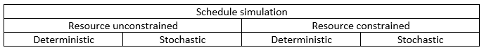
Project schedule simulation was run in four modes.  We were concerned with differences in expected duration, task criticality and finish time correlation between resource unconstrained and constrained schedule simulations   Primarily, schedules were either resource unconstrained or constrained.    Secondarily, task durations were treated deterministically or stochastically.  The modes are summarized in Table 1.

Table 1.  Simulation modes

An example

Figure 1 shows a project schedule with over allocated resources.  It is unleveled.  There is one unit of each resource type.   The set of logical dependencies is A= [(0, 2), (3, 4), (3, 5), (6, 7), (7, 8)].  The results of all four simulation modes is presented below.  For each mode, a simulation was run with 10,000 trials.

Figure 1.  Example: over allocated (unleveled) project schedule

Deterministic resource unconstrained case

This case reduces to the simple CPM result.  Project duration is 15 days and the CP is (6,7,8).  Since task duration and logical dependencies are constant, the result is always the same.   Table 2 shows CP frequency. 

Table 2.  Critical path set frequency, resource unconstrained, deterministic case

Deterministic resource constrained case

There are four distinct non-delay resource-feasible schedules, each identified by a unique vector of task start times:  a 16-day schedule, two 22-day schedules and a 26-day schedule.  Figure 2 is a stacked histogram showing the sample proportion of the four non-delay resource-feasible schedules, along with their associated task start time vectors (sVec).

Figure 2.  Non-delay resource-feasible schedule frequency (n=10,000)

In this example, since there is only one unit of each resource type, the sets of resource constraints are limited.  There is only one set of resource constraints associated with each start vector.  Hence, in this example, each start vector will be associated with only one unique RCP set.  Both 22-day schedules have the same RCP set.  Table 3 shows RCP set frequency.  

Table 3.  RCP set frequency, resource constrained, deterministic case (n=10,000)

If a set of resource constraints is added to the set of logical constraints in MS Project, we can visualize the resource-feasible schedule with its RCP’s identified.  All four of the resource-feasible schedules share the logical constraints:  A= [(0, 2), (3, 4), (3, 5), (6, 7), (7, 8)].  Figures 3-6 show these schedules.  The vector of task start times (sVec), the set of resource constraints (A_R), and the RCP are included in each figure.  As mentioned above, phantom float, a normal byproduct of resource leveling, is eliminated when the union of logical and resource constraints drives task sequencing.  Examination of these four schedules will be instructive when we discuss finish time correlation in a later section.

Figure 3.  16-day non-delay resource feasible schedule

Figure 4.  22-day non-delay resource-feasible schedule (a)

Figure 5.  22-day non-delay resource-feasible schedule (b)

Figure 6.  26-day non-delay resource feasible schedule

Stochastic resource unconstrained case

Figure 7 shows the frequency distributions of project durations for both the stochastic resource unconstrained and constrained cases.  Figure 8 shows the mean and cumulative frequency distribution of project durations for both the stochastic resource unconstrained and constrained cases.    The difference between the resource unconstrained and constrained cases is clear. 

In the stochastic resource unconstrained case the mean project duration is 15.76 days.  As compared to the deterministic duration of 15 days, the increase is attributable to accumulated merge bias, an effect seen when paths converge in the schedule network. 

Figure 7.  Project duration frequency distributions for resource unconstrained and constrained simulations (n=10,000)

Figure 8.  Expected project durations and cumulative frequency distributions for resource unconstrained and constrained cases (n=10,000)

Table 4 shows the CP set frequency for the stochastic resource unconstrained case.  The CP identified in the resource unconstrained deterministic case is found to be dominant in the stochastic case.  As task durations varied, there were relatively few trials in which a different CP emerged.

 Table 4.  CP set frequency, stochastic resource unconstrained case

Stochastic resource constrained case

Simulation of resource constrained schedules allows us to measure the difference between expected duration in resource unconstrained and resource constrained schedules. Referring to Figure 8 above, the mean project duration in the stochastic resource constrained case shifts to 22. 59 days.  This shift is primarily caused by the imposition of resource constraints, and secondarily, merge bias (when compared to the deterministic weighted mean project duration of 21.40 days, from Figure 2).

The cumulative frequency distributions (CFD’s) from Figure 8 allow us to determine the likelihood of meeting a certain project finish time.  While the deterministic 16-day leveling appears to be optimal in terms of schedule duration, the likelihood of achieving it is minimal.  It is far more likely that the project will take 22 days or more to complete. 

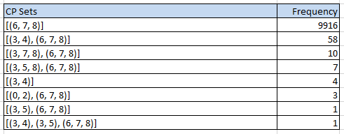
Table 5 shows RCP set frequency.  There are 59 distinct RCP sets, with the RCP associated with the 22-day resource-feasible schedules being dominant.  In this sampling, the original CP of (6,7,8) does not occur!

Table 5.  RCP set frequency, stochastic resource constrained case

Criticality

The set of CP’s or RCP’s is recorded for each simulation trial.  As was seen above, there can be more than one CP or RCP for any given schedule.  A task’s criticality is the proportion of trials in which the task is a member of a CP or RCP in the set.  It represents the likelihood that the task is critical.  Table 6 shows the proportions for each simulation mode.  Considering only the stochastic cases, Figure 9 plots the proportions to facilitate comparison. 

In this particular resource unconstrained simulation, the critical path was (6,7,8) in 99.16% of the trials.  Whereas, the resource constrained simulation shows the dominance of the tasks associated with the 22-day resource-feasible RCP, (3,2,7,8).   The dominant resource critical path set [(3,2,7,8)] determined the project duration in 53.66% of the trials in this particular resource constrained simulation. 

Table 6.  Criticality proportions for each simulation case

Figure 9.  Criticality proportions for stochastic simulation cases

Finish time correlation

For each trail in the simulation, task finish times and the project finish time were recorded.  Spearman’s rank order correlation coefficients were calculated to measure the relationship of task and project finish times in the simulation sample.  Since the relationship between a task’s finish time and the project finish might not be linear, a rank order correlation statistic was used. 

Table 7 shows the finish time correlation coefficients.  In the table, blank cells are not defined.  In the deterministic resource unconstrainted case, the project finish time and all task finish times are constant.  In the deterministic resource constrained case, this is partially so.  Considering only the stochastic cases, Figure 10 plots the coefficients to facilitate comparison.

Table 7.  Finish time correlations for resource unconstrained and constrained simulations (n=10,000)

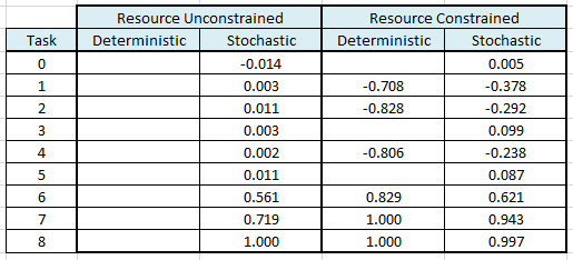
Figure 10.  Finish time correlations for resource unconstrained and constrained simulations (n=10,000)

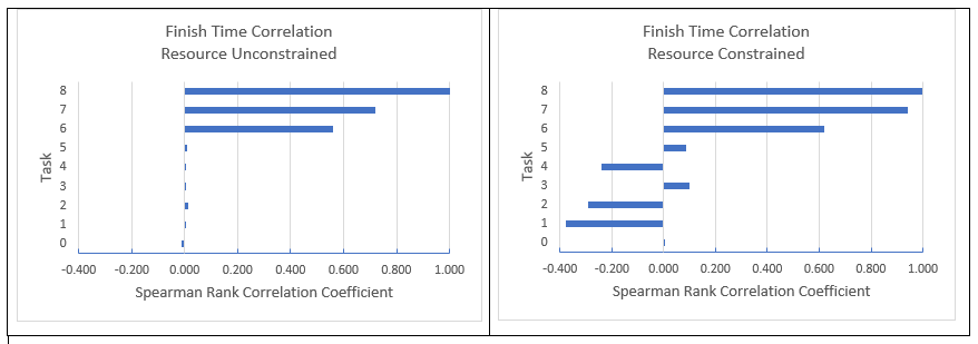
In the stochastic resource unconstrained case, the finish times of tasks 6, 7 and 8 are positively correlated with the overall project finish time.  These tasks are members of the dominant critical path in the resource unconstrained case.  If these tasks finish later, it is likely that the project will finish later.   Task 8 has the strongest correlation.  If the finish of 8 is delayed, there is little that can be done to recover, since that is the last task in the CP.  Whereas, if tasks 6 or 7 finish late, this might be compensated for with later tasks finishing early.

In the stochastic resource constrained case, the finish times of tasks 6, 7 and 8 are positively correlated with the overall project finish time.   In addition, task 1 has a moderate negative correlation.  If task 1 finishes early, then the project will finish later.  In reviewing the deterministic resource constrained schedules above (Figures 3-6), task 1 starts at the beginning time in the 26-day and one of the 22-day schedules, whereas, it starts later in the 16-day and the other of the 22-day schedules.  The sooner is starts (and finishes), the longer the overall schedule finish time.  Tasks 2 and 4 have negative correlations, as well.  Task 2 is scheduled later in the shorter 16-day schedule and task 4 is scheduled earlier in the longer 26-day schedule. 

In the resource constrained case, there is much more complexity.  Task finish times are both positively and negatively correlated with the project finish time.  And, more than just the dominant resource critical tasks are involved. 

Conclusions

In this example, we saw that there were differences between the resource unconstrained and constrained simulation results. 

• The expected project duration was greater in the resource constrained schedules than in the resource unconstrained schedule, primarily due to the imposition of resource constraints.
• Whereas task criticality mirrored the dominant CP in the resource unconstrained schedule, it mirrored the dominant RCP in the set of constrained schedules.
• Finish time correlations were aligned with the dominant CP in the unconstrained case but there were both postive and negative correlations in the resource constrained case, involving tasks not aligned with the dominant RCP. 

In presenting project duration estimates, it is prudent for a project manager to assess the impact that resource constraints have on expected project duration, task criticality and task finish time correlation.

_____________________

© Nicklas, Inc. and robinnicklas.com, 2019.  All rights reserved.  Unauthorized use and/or duplication of this material without express and written permission from this site’s author and/or owner is strictly prohibited.