In the first of this series of articles on modeling project stakeholder networks using social network analysis, we showed how stakeholder networks could be displayed as graphs. In this article, we will explore how changes in network topology affect centrality and community. Both concepts describe how stakeholders are connected to each other. This connectivity determines how information flows through a network and the degree to which an individual stakeholder or a group of stakeholders controls that flow.
Centrality and community measures
There is a general notion that the more central a node is, the more influential it is. A stakeholder in a central position can regulate the flow of information through the network. Such a stakeholder has more direct access to other stakeholders and has increased visibility and importance relative to their position in the network. Further, there is a notion that community affects the flow of information between groups of nodes in the network.
There are several ways to measure the centrality of a node (vertex) in a network. Degree centrality is a simple count of how many other nodes a particular node is directly connected to. Closeness is the average path distance from a particular node to other nodes. Nodes with low closeness receive information sooner and can disseminate it faster than other nodes. Betweenness measures the number of paths between any two other vertices that pass through a particular vertex. Nodes with high betweenness see a higher volume of network traffic and they can control the flow of information. Eigenvector centrality measures how close a particular node is to other highly connected nodes. The greater the value, the better connected the node is. We will use the latter measure of centrality in this article. See Borgatti (2005), Hanneman (2005) and Ognyanova (2016) for a discussion of these centrality measures.
Community is a measurement of how closely groups of nodes are connected to each other. Being the member of a community implies that members of a group are more closely connected to other members in the group than to members of other groups. The more tightly connected a group of nodes is, the flow of information between groups might be affected. Also, it is more likely that individuals within a group are homophilic or like-minded. Cliques are an extreme case where all members of a group are connected to all other members of the group. Clustering measures how likely it is that two of a stakeholder’s connections are themselves connected. The walktrap algorithm for measuring community assumes that nodes encountered on short random walks from a given node are likely to be members of the same group. See Pons and Latapy (2005) for a discussion of the algorithm. We will use this algoritihm as the measure of community in this article.
For a good, general discussion of how network structure affects power and influence, see Easley and Kleinberg (2010).
Networks change over time
Networks are not static. They change over time. This means that centrality and community measures change over time as network topology changes. There are two ways you can change a network: add or remove nodes and add or remove edges. Adding or removing stakeholders on a project changes the underlying network topology and can shift the balance of influence a stakeholder has. Increasing or decreasing the number of communication channels amongst the stakeholders promotes or hinders collaboration amongst the stakeholders.
The case study used in this series of articles is described in a prior article. In this article, three network states will be explored. The first is the network state prior to the addition of the consulting project manager. The second is the network state after the PM is introduced. And, the third is the network state after the PM and vendor Account Manager collaborate to strengthen ties between the three groups of IT staff. Between the first and second state, a key stakeholder is added. Between the second and third state, additional communication channels are established between the geographically dispersed IT groups.
In an attempt to bolster the status of the desktop imaging project, the Network VP introduced a Project Manager into the mix. The PM collaborated with the vendor Account Manager to arrange a field trip to the vendor site in order to encourage communication between key staff members in each of the three IT groups. In essence, the Network VP and PM are building coalitions of stakeholders that want to see the project succeed. In the process, they are diminishing the influence of stakeholders that may not want the project to succeed.
Changes in centrality
Figure 1 shows how centrality changes over the three network states. Table 1 shows the specific eigenvector centrality measures for each stakeholder node across the three network states. In the figure, node size and color intensity reflect eigenvector centrality. It is interesting to compare node size in this figure to the original network graph (see the prior article) in which node size indicated organizational power relative to reporting relationships in the organization chart.
We can see that there is a clear shift in centrality from the Director IT to the Project Manager over the three states. And, the IT Strategist’s centrality decreases, diminishing the effect of her antagonism against the project. Further, as collaboration amongst the IT groups is encouraged, we see that the centrality of the IT groups, including the vendor group, increases.
In the centrality and community calculations used in this article, all network edges are undirected and unweighted. Only communication channels are considered. The reporting and personal relationships included in the prior network graph are not considered.
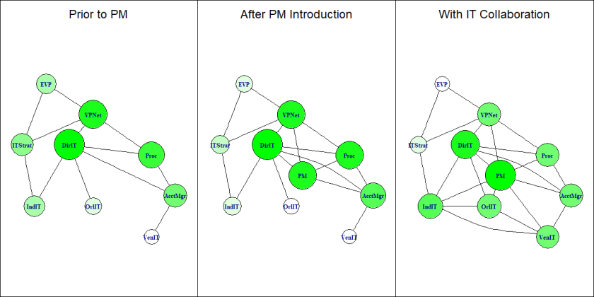
Figure 1. Shift in eigenvector centrality as network topology changes. Larger node size and darker color intensity indicate larger values.

Table 1. Eigenvector centrality for each node in each network state
Changes in community
Figure 2 shows the shift in community membership over the three network states. Whereas there were three distinct communities in the initial state, with the vendor and Orlando IT groups being somewhat isolated, there are just two communities once the PM is introduced. And, after the PM and Account Manager promote IT group collaboration, the former Iota IT group is drawn into the project community under the control of the PM.
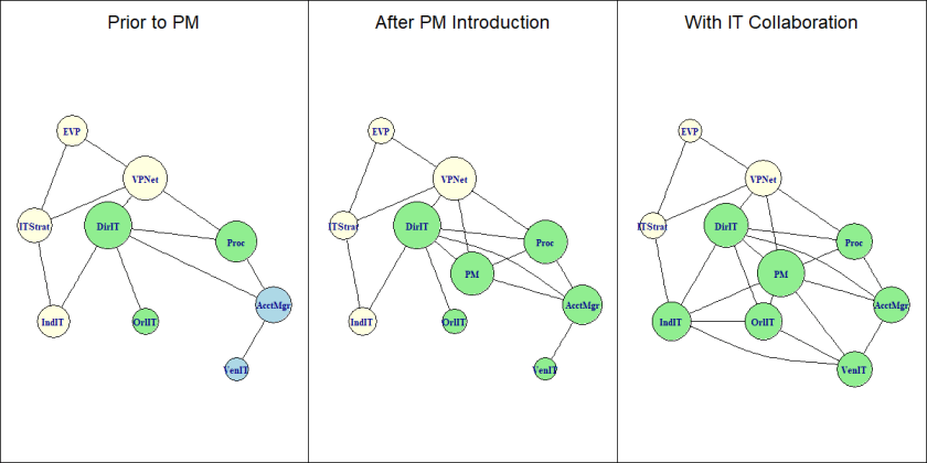
Figure 2. Shift in walktrap community membership as network topology changes. Node color indicates community membership. Larger node size indicates larger eigenvector centrality.
Summary
The objective of stakeholder management is to build (or, in some cases destroy) coalitions, which are groups of stakeholders with linked agendas or interests. From the transitions in centrality and community above, we see that specific changes to network topology — adding nodes or increasing connections—can change node centrality and community measures over time. In the case study, when the Network VP introduced the Project Manager, it shifted power away from the primary antagonist, the IT Strategist. When the PM worked with the vendor Account Manager to improve collaboration amongst the IT groups, it made the PM the central figure rather than the Director IT. As the PM acquired power and built a coalition, the Executive VP, IT Strategist, and to some extent the Network VP were isolated from the rest of the project team. The former Iota IT group was drawn into the main project community around the centralized PM.
Bilbiography
Borgatti, S. P. (2005). Centrality and network flow. Social Networks, 27, 55-71.
DeLuca, Joel M. Political Savvy. (1992). Horsham, PA: LRP Publications.
Easely, David and Jon Kleinberg. Networks, Crowds, and Markets: Reasoning about a Highly Connected World. Cambridge University Press, 2010. (Draft version) Web. 13 September 2015 (https://www.cs.cornell.edu/home/kleinber/networks-book/networks-book.pdf)
Hanneman, R. A., & Riddle, M. (2005). Introduction to social network methods. Riverside, CA: University of California, Riverside. (http://faculty.ucr.edu/~hanneman/; retrieved 6 June 2018)
Ognyanova, K. (2016). Network Analysis and Visualization with R and igraph: NetSci X Tutorial. (http://www.kateto.net/networks-r-igraph; retrieved 6 June 2018)
Pons, Pascal and Matthieu Latapy. (2005). Computing communities in large networks using random walks. (http:// arXiv:physics/0512106; retrieved 18 June 2018)
________________
© Nicklas, Inc. and robinnicklas.com, 2018. All rights reserved. Unauthorized use and/or duplication of this material without express and written permission from this site’s author and/or owner is strictly prohibited.
