A prior article demonstrated that for an unleveled project schedule, there could be multiple, non-delay resource-feasible schedules of varying durations. The range, distribution and mean of this set of durations could be estimated using simulation. Further, it was demonstrated that for any particular resource-feasible project duration in the set of non-delay schedules, there could be multiple, unique resource-feasible schedules that would yield that particular project duration.
A different article showed how to identify resource critical paths and remove phantom float errors in resource-leveled schedules. In the simple example used in that article, the capacity of each resource type was limited to one unit. That simplified the identification of resource paths and constraints. However, projects usually have more than one resource type and more than one unit of each type. This complicates the identification of the resource paths and constraints required to identify resource critical paths. Since there can be multiple sequences describing how a unit resource is assigned to tasks, there can be more than one set of resource constraints derived from a unique resource-feasible schedule. And, there can be more than one combination of resource critical paths for that unique resource-feasible schedule.
In this article, we will explore this ambiguity using simulation. First, we will generate sets of resource paths that can be used to define sets of resource constraints for a unique resource-feasible schedule. Then, using these sets of resource constraints, we will identify the combinations of resource critical paths that are derived from these sets of resource constraints.
Resource paths and resource constraints
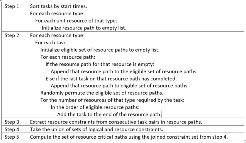
A resource path is the sequence of tasks to which a particular unit resource is assigned. A resource path is synonymous with resource flow or resource chain. Algorithm 1 constructs resource paths for a resource-feasible project schedule. Steps 1 and 2 construct resource paths for each individual resource within a resource type. The steps were adapted from algorithms found in Policella, et. al. (2007) and Deblaere, et. al. (2007).
The algorithm starts by sorting tasks according to their start times in the resource-feasible schedule. For each task in start-time order, the set of eligible resource paths that the task could draw resources from is determined. Each unique resource has its own path. Eligible resource paths are those on which no task has been assigned or on which the last task assigned has been completed. In this study, the eligible set of paths is randomly permuted. Following that random order, the task is appended to as many eligible resource paths as the task requires. Each time the algorithm is invoked, it will generate a set of resource paths, at random. If the algorithm is invoked multiple times, sets of resource paths are generated.
A set of resource constraints are extracted from a set of resource paths. Each successive pair of tasks in a resource path represents a resource constraint. For that resource, one task must finish before the next task can start. The extraction of resource constraints is accomplished in step 3 of the algorithm. Step 4 joins the set of resource constraints with the set of logical constraints. The set of non-redundant resource constraints AR is the difference of the set of combined constraints and the set of logical constraints. In other words, there may be some resource constraints that are also logical constraints, and hence, redundant.
Algorithm 1. Resource path generation for a resource-constrained schedule
Resource critical paths (RCPs)
By joining the set of non-redundant resource constraints AR and the set of logical constraints A, the set of RCPs for the unique schedule can be calculated. The set of RCPs is small relative to the size of the set of resource constraint sets. For the unique resource-feasible schedule, there is a set of combinations of RCPs for that schedule. Some sets of resource constraints will yield one combination of RCPs, while another set of resource constraints will yield a different combination of RCPs, or perhaps a single RCP. The percentage of trials in which a certain combination of RCPs occur can be estimated.
Resource critical path ambiguity
Figure 1 summarizes the resource leveling and allocation process used to identify the set of resource critical path combinations for a unique resource-feasible schedule. The figure shows three points of ambiguity: for an unleveled schedule, there can be a distribution of unique resource-feasible schedules; for any unique resource-feasible schedule, there can be multiple sets of resource constraints that describe how resources can be allocated to tasks; and, for a set of sets of resource constraints, there are a limited number of combinations of resource critical paths defined by that set.

Figure 1. Resource critical path identification for unique resource-feasible schedules
Starting with an unleveled schedule, tasks are scheduled relative to resource constraints. Simulation was used to identify and describe the distribution of resource-feasible schedules. The distribution exists over a range of schedule durations. And, for any duration in that range, there can be multiple unique schedules that yield that duration. This is the first point of ambiguity. For any unleveled schedule, there can be multiple resource-feasible schedules, the likelihood of which can be determined through schedule simulation taking resource constraints into account. This was shown in a prior article.
The second point of ambiguity results from the way in which resources are allocated in resource-feasible schedules. For any unique resource-feasible schedule, there can be any number of ways in which resources are assigned to tasks in that schedule. Simulation was used to generate sets of resource paths that describe how individual resources are assigned to tasks. There can be multiple unique sets of resource paths generated from one unique resource-feasible schedule. A set of resource constraints is extracted from a set of resource paths. Hence, there can be multiple sets of resource constraints describing how resources are allocated in a resource-feasible schedule.
The set of resource constraints is joined with the set of logical constraints to compute resource critical paths (RCPs). The set of resource-constraint sets reduces to combinations of a set of RCPs and that the likelihood of any combination can be determined through simulation. This is the third point of ambiguity.
Figure 1 shows how we get from an unleveled schedule to a combination of RCPs describing how resources might be leveled and allocated for that schedule. Further, the figure shows how expansive the problem is. The Resource Constrained Project Scheduling Problem (RCPSP) is NP-Hard. By using simulation, we can reduce the set of resource constraint sets for a unique resource-feasible schedule to a set of combinations of RCPs. And, we can assess the large number of possible outcomes that exist for any unleveled schedule by describing the range and likelihood of the distribution of resource feasible schedules.
An example
We will continue to use the resource-constrained schedule from Deblaere, et. al. (2007) that we used in the prior articles. The unleveled schedule is presented in Figure 1. The critical path is <1,5,8> and the schedule is 13 days long. The set of logical constraints is A = {<0,4>,<1,5>,<2,6>,<3,7>,<5,8>}. There is only one resource type r, and r’s capacity is 10.
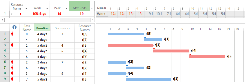
Figure 2. Unleveled schedule, from Deblaere (2007)
There are four 13-day, active, resource-feasible schedules for this instance, as identified by their unique task start-time vectors (sVec). There are other active, resource-feasible schedules of greater duration, but those will not be discussed here. Figure 3 shows the leveling and allocation results for these four resource-feasible schedules. We will start with the one presented in Deblaere (2007), sVec = <0,0,0,6,4,5,2,8,9>, and will then compare it to the other three. We can see that each resource-feasible schedule generates its own set of RCPs. While two of the schedules generate combinations of RCPs, the other two generate just one RCP, which is equivalent to the original logical critical path.

Figure 3. Example resource critical path identification for four active, resource-feasible schedules
sVec = <0,0,0,6,4,5,2,8,9>
This instance yields two combinations of RCP’s. In both combinations, the logical critical path, <1,5,8> is present. It represents the lower limit of the resource-feasible schedule length. A second RCP, <0,4,3,7>, is present, with the logical CP, in 29% of the trials. However, in 71% of the trials, a third RCP, <2,6,4,3,7>, is present with the other two RCPs. In the latter case, all tasks are resource critical.
To represent these two outcomes, one set of resource constraints yielding each outcome was arbitrarily selected from the set of unique sets of resource constraints generated by the simulation. These sets of resource constraints AR were added to the set of logical constraints A to generate a schedule showing RCPs. This method was described in a prior article. Figure 4 shows the two RCP combination and Figure 5 shows the three RCP combination.

A = {<0,4>,<1,5>,<2,6>,<3,7>,<5,8>} AR = {<0,3>,<0,5>,<1,3>,<4,3>,<6,5>,<6,8>} RCP = {<0,4,3,7>,<1,5,8>}
Figure 4. sVec = <0,0,0,6,4,5,2,8,9>, two RCP combination (29% frequency, n=10,000)
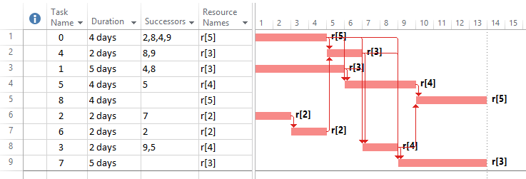
A = {<0,4>,<1,5>,<2,6>,<3,7>,<5,8>} AR = {<0,3>,<0,5>,<0,7>,<1,3>,<3,8>,<4,3>,<4,7>,<6,4>} RCP = {<0,4,3,7>,<1,5,8>,<2,6,4,3,7>}
Figure 5. sVec = <0,0,0,6,4,5,2,8,9>, three RCP combination (71% frequency, n=10,000)
sVec = <7,0,0,0,11,5,2,2 9>
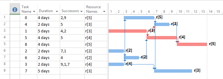
For this instance, a two RCP combination occurred in 30% of the trials and a three RCP combination occurred in 70% of the trials. The set of RCPs, {<1,5,8>,<2,7,0,4>,<3,7,0,4>}, is different from the set in the first instance, {<0,4,3,7>,<1,5,8>,<2,6,4,3,7>} . The two combinations are shown in Figures 6 and 7.

A = {<0,4>,<1,5>,<2,6>,<3,7>,<5,8>} AR = {<1,0>,<3,5>,<6,0>,<6,5>,<7,0>,<7,8>} RCP = {<1,5,8>,<3,7,0,4>}
Figure 6. sVec = <7,0,0,0,11,5,2,2 9>, two RCP combination (30% frequency, n=10,000)

A = {<0,4>,<1,5>,<2,6>,<3,7>,<5,8>} AR = {<2,7>,<3,0>,<3,6>,<6,5>,<6,8>,<7,0>} RCP = {<1,5,8>,<2,7,0,4>,<3,7,0,4>}
Figure 7. sVec = <7,0,0,0,11,5,2,2 9>, three RCP combination (70% frequency, n=10,000)
sVec = <2,0,0,0,6,5,2,6,9>
In this schedule, the RCP is always <1,5,8>, which is the same and the original logical CP. The schedule is displayed in Figure 8.
A = {<0,4>,<1,5>,<2,6>,<3,7>,<5,8>} AR = {<0,7>,<1,4>,<2,0>,<3,0>,<3,6>,<4,8>,<6,5>} RCP = {<1,5,8>}
Figure 8. sVec = <2,0,0,0,6,5,2,6,9>, single RCP (100% frequency, n=10,000)
sVec = <0,0,0,4,6,5,2,6,9>
In this schedule, the RCP is always <1,5,8>, as well. Figure 9 displays the schedule. The cardinality of the set of unique sets of RCs is relatively small compared to the other schedules presented.

A = {<0,4>,<1,5>,<2,6>,<3,7>,<5,8>} AR = {<0,3>,<0,5>,<0,7>,<3,4>,<4,8>,<6,3>} RCP = {<1,5,8>}
Figure 9. sVec = <0,0,0,4,6,5,2,6,9>, single RCP (100% frequency, n=10,000)
The temporal nature of resource constraints
In a typical project lifecycle, there are two primary places where a schedule is leveled. Towards the end of the planning phase, the entire schedule is leveled to ensure it is resource-feasible prior to setting a schedule baseline. And, at the end of each tracking cycle, a schedule is leveled from the status date through the end of the schedule to ensure that the remaining schedule is resource-feasible.
However, a lot can happen to a schedule between these leveling points. In a prior article, we used schedule simulation to mimic these perturbations, by treating task duration as a random variable. As task durations change, the leveling can change, as well. Any perturbation during project execution can divert the leveling and allocation from one solution to another. While a particular set of resource constraints yields a particular combination of RCPs, all it takes is a perturbation in a task duration and the set of resource constraints changes, which may lead to a different set of RCPs. Resource-constraints and RCPs, like phantom float, are byproducts of the leveling process. They are dependent on the leveling. And, they can change frequently throughout schedule execution.
While we can discover the RCPs for a unique resource-feasible schedule, the likelihood of them changing due to perturbations in task durations is high. Hence, RCPs and the other leveling artifacts are ephemeral—they can change continually throughout the execution of a project.
Summary
Using simulation, we generated a set of unique resource-feasible schedules from an unleveled project schedule. The set of resource-feasible schedules is distributed over a range of project durations. For a unique resource-feasible schedule in this set, simulation was used to generate a set of resource path sets representing the variety of ways in which unique individual resources could be allocated in that schedule. Non-redundant resource constraint sets were extracted from the sets of resource paths. Each unique set of non-redundant resource constraints was joined with the original set of logical constraints to compute a set of schedules in which resource critical paths were identified. For a unique resource-feasible schedule, combinations of resource critical paths were identified. The frequency at which these combinations occur can be estimated.
References
Deblaere, Filip and Erik Demeulemeester, Willy Herroelen, Stijn Van De Vonder. 2007. “Robust Resource Allocation Decisions in Resource-Constrained Projects.” Decision Sciences. 38 (1): 5-37.
Policella, Nicola; Amedeo Cesta; Angel Oddi; Stephen F. Smith. 2007. “From Precedence Constraint Posting to Partial Order Schedules: A CSP approach to Robust Scheduling.” AI Communications. 20 (3), 163-180.
________________
© Nicklas, Inc. and robinnicklas.com, 2018. All rights reserved. Unauthorized use and/or duplication of this material without express and written permission from this site’s author and/or owner is strictly prohibited.
