Whenever we use project scheduling software, such as Microsoft Project, to level resources in a schedule, we get a single solution. However, being presented with just one resource leveling solution can be misleading. For any unleveled project schedule, there is an infinite number of resource-feasible schedules. Generally, we try to limit the set of solutions and then search for an optimal schedule. Usually, we search for a schedule that has the shortest project duration after resource leveling. In this article, rather than search for an optimal resource-feasible schedule, we will explore the use of simulation as a means of identifying and describing a subset of resource-feasible schedules. Once we can visualize a set of resource-feasible schedules, we can better assess the solution that is produced by the scheduling software.
Semi-active, active and non-delay schedules
Searching an infinite set of resource feasible schedules is not a good idea. We need to reduce the solution set to a manageable size. The first step in culling the solution set is to limit the set to resource feasible schedules in which all tasks are scheduled as soon as possible relative to any logical and individual resource constraints. The result is the set of semi-active schedules. The second step is to limit the set to resource feasible schedules in which no task can be scheduled earlier without delaying some other task or violating a logical or resource constraint. This is the set of active schedules and it is a subset of the semi-active schedules. If we are searching for an optimal schedule duration, for example, it will be found in the set of active schedules. The set of non-delay schedules are resource-feasible schedules in which no individual resource is left idle if it can be assigned to a task that is eligible to be scheduled relative to logical and resource constraints. The set of non-delay schedules is a subset of active schedules. However, the non-delay set might not contain an optimal solution. For further information about schedule classification, see Baker and Trietsch (2009) or Brucker (2007).
There are schedule generation schemes for exhaustively enumerating the set of active schedules. And, there are sophisticated strategies to search for optimal solutions, such as branch and bound techniques or genetic algorithms. However, since the set of active schedules could be quite large, it might be time-consuming, if not impractical, to find an optimal solution. To get around this problem, project scheduling software uses dispatching algorithms with a set of heuristics (leveling rules) to resource level a schedule. While this is a quick method of finding a single solution, it is not guaranteed to yield an optimal solution.
In this article, we start with a dispatching process that produces a single resource-feasible, non-delay schedule. The process uses random permutation to decide which tasks are assigned resources at each decision point in the scheduling process. The process is run multiple times to generate a sample of resource-feasible, non-delay schedules. Once we have the sample, we can characterize the distribution of project durations and identify unique solutions. Rather than exhaustively enumerate the solutions, we use simulation to approximate the solution set and its distribution.
A simple leveling algorithm
The steps in Algorithm 1 outline a single-pass, parallel dispatching process that generates a single non-delay resource-feasible schedule. In Step 3, instead of using typical leveling heuristics, such as minimum float, minimum duration or task ID, the eligible set is randomly permuted. This approach is myopic in the sense that it does not consider additional information that requires recomputing the schedule (float) or looking ahead (greatest number of remaining tasks or resources used). In the algorithm, each task in the set of project tasks is assigned a mutually exclusive status: unscheduled, scheduled (in progress), and completed. All tasks start in the unscheduled state. At the end, all tasks have been scheduled.
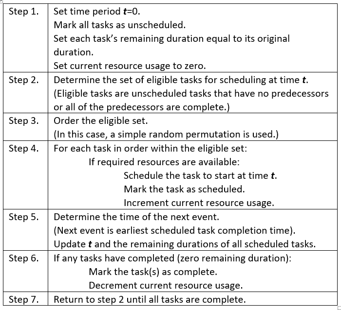
Algorithm 1. Non-delay resource-feasible schedule generation
As in prior articles, we have simplified the resource-constrained scheduling problem by prohibiting preemption (splitting tasks) and the adjustment of initial assignment units (multi-tasking). This algorithm is not intended to yield an optimal solution. Rather, it generates a single member of the non-delay schedule set, at random. See Kolisch (1996) or Vanhoucke (2012) for a review of serial and parallel schedule generation algorithms. While a single-pass, serial schedule generation scheme generates active schedules, we will limit our discussion in this article to non-delay schedules generated through a parallel scheme.
Simulation
If the leveling algorithm is invoked multiple times, a random sample of non-delay schedules is generated. Note, we are not sampling from the non-delay set. We don’t know in advance what that set is. Rather, we are generating a sample of randomly generated non-delay schedules and then using that sample to characterize the non-delay set. Each invocation of the algorithm is called a trial. A simulation could entail the generation of thousands of trials. The project duration and start time vector for each trial is recorded. At the end of the simulation, the resulting distribution of project durations can be described, the set of unique start time vectors identified, and the cross tabulation of project durations and start vectors ascertained. This will allow us to see what the solution set of resource-feasible schedules looks like.
An example
Let’s use a resource-constrained schedule from Deblaere, et. al. (2007). The unleveled schedule is presented in Figure 1. The critical path is <1,5,8> and the schedule is 13 days long. The set of logical constraints is A = {<0,4>,<1,5>,<2,6>,<3,7>,<5,8>}. There is only one resource type r, and r’s capacity is 10. The schedule requires 108 resource-days of work. With 130 resource-days available within a 13-day schedule, it is not impossible for a 13-day resource-feasible schedule to be found. The schedule cannot be shorter than 13 days since that is the length of the logical critical path.

Figure 1. Unleveled schedule (adapted from Deblaere, et. al. (2007)).
A simulation with 10,000 trials was run. The distribution of non-delay leveled project durations is shown in Figure 2. The cross tabulation of project durations and unique start vectors is shown in Figure 3.

Figure 2. Proportion of non-delay schedule durations, n=10,000 trials
We see that there is a small number of unique resource-feasible project durations over a range of resource-feasible project durations. The notion that you can have a range of resource-feasible project durations is easily missed when project scheduling software returns just a single solution. Knowing the distribution of leveled schedule durations, you can assess where the single solution provided by the scheduling software is positioned relative to the range of durations. In this example, the mean project duration of resource-feasible schedules is longer than the duration of the unconstrained schedule. It will never be shorter than the length of the unleveled schedule. The difference between the unleveled schedule duration and the mean of non-delay schedules is an estimate of the average schedule delay caused by tasks being blocked, waiting for resources in this particular example.
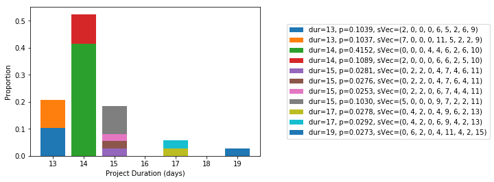
Figure 3. Proportion of unique non-delay leveled schedules by project duration
We see that there is a limited set of unique non-delay leveled schedules. And, for each unique resource-feasible project duration, we see that there can be multiple unique non-delay schedules that yield that duration. For example, there are four unique schedules that generate at 15-day schedule. In this example, we see that schedules 14-days or longer in duration are roughly four times more likely to occur than 13-day schedules.
Optimal schedules
For this example, there are two 13-day, non-delay solutions. The first has a vector of task start times, sVec = <2,0,0,0,6,5,2,6,9>. It happens to be the 13-day schedule generated by MS Project 2016 using the Standard leveling order. The other has a vector of task start times, sVec =<7,0,0,0,11,5,2,2,9>. This means that there is more than one optimal resource-feasible schedule.
MS Project 2016, using the ID only leveling order, generates a 13-day resource-feasible schedule with start time vector sVec = <0,0,0,6,4,5,2,8,9>. This is the resource-feasible schedule treated in the DeBlaere article mentioned above. While it is an active schedule, it is not a non-delay schedule and is not discussed here.
The two non-delay schedules are shown in Figures 4 and 5. These schedules are displayed in MS Project by manually inserting Leveling Delay (lag) in front of any task that was delayed due to a resource constraint. Resource critical paths were not identified.

Figure 4. Non-delay schedule with task start time vector sVec = <2,0,0,0,6,5,2,6,9>
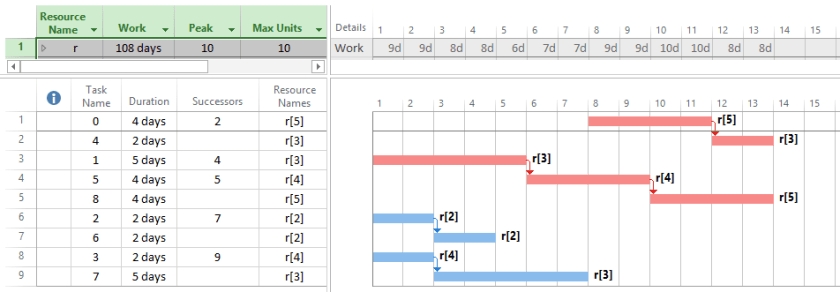
Figure 5. Non-delay schedule with task start time vector sVec = <7,0,0,0,11,5,2,2,9>
Standard error of mean project duration
To assess the affect of sample size on the simulation results, we look at three measures: number of unique project durations, number of unique resource-feasible non-delay schedules, and the mean project duration. Samples of simulations consisting of 100, 1000, 2000, 5000 and 10000 trials were generated. The number of unique project durations (five, in this example) and number of unique non-delay schedules (eleven, in this example) both stabilize at 1000 trails and remain constant thereafter. Simulations of 100 trials were not sufficient. Figure 6 charts the estimate and confidence interval of the mean non-delay schedule duration by the number of trials in a simulation. As the number of trials increases, the estimate of the average project duration converges, as would be expected.

Figure 6. Mean non-delay schedule duration by number of simulation trials
The purpose of the algorithm is to demonstrate how we can use simulation to describe the set on non-delay schedules for a simple, small example. The efficiency of the method and how it scales to larger, more complex projects has not been addressed.
Conclusions
There are a few important observations. First, there is a distribution of resource-feasible, non-delay schedule durations. Second, the mean non-delay schedule duration can be estimated. The difference between the unleveled schedule duration and the mean non-delay schedule duration is an estimate of how much the schedule is delayed due to resource blockage. And third, for each unique non-delay schedule duration, there can be multiple unique non-delay schedules (unique start time vectors) that yield that duration.
Being able to visualize and describe the distribution of resource-feasible schedules helps us assess the single solutions presented by scheduling software. In the example, there are three active 13-day, resource-feasible schedules, two of which are non-delay schedules. MS Project’s ID only leveling order produced an active schedule that was not a member of the non-delay set. MS Project’s Standard leveling order produced one of the two non-delay schedules. However, if we look at the distribution of resource-feasible, non-delay schedules, we see that 14-day or longer schedules are approximately four-times as likely to occur than the 13-day optimal solution.
References
Baker, Kenneth R. and Dan Trietsch. 2009. Principles of Sequencing and Scheduling. Wiley.
Brucker, Peter. 2007. Scheduling Algorithms (5th edition). Springer.
Deblaere, Filip and Erik Demeulemeester, Willy Herroelen, Stijn Van De Vonder. 2007. “Robust Resource Allocation Decisions in Resource-Constrained Projects.” Decision Sciences. 38 (1): 5-37.
Kolisch, Ranier. 1996. “Serial and Parallel Resource-Constrained Project Scheduling Methods Revisited: Theory and Computation.” European Journal of Operational Research. 90:320-333.
Vanhoucke, Mario. 2012, January 10. “Optimizing Regular Scheduling Objectives: Schedule Generation Schemes.” Retrieved from http://www.pmknowledgecenter.com/dynamic_scheduling/baseline/optimizing-regular-scheduling-objectives-schedule-generation-schemes.
________________
© Nicklas, Inc. and robinnicklas.com, 2018. All rights reserved. Unauthorized use and/or duplication of this material without express and written permission from this site’s author and/or owner is strictly prohibited.
